Capstone: Building a Cumulative-Burden Index from the Data Up

The question

New Jersey’s Environmental Justice Law rests on the idea of cumulative burden: many pollution sources and stressors adding up in the same places. NJDEP measures this by counting how many of 26 stressors are above a comparison point (the Combined Stressor Total, or CST; see my post on the appeals court ruling and my Supreme Court post). Counting is simple and transparent, but it treats every stressor as equally important and ignores how far above the line a community is.

For this capstone post, I asked: if we let the data reveal their own structure, without a pre-set counting rule, what does cumulative burden look like in New Jersey? And does it agree with the official approach?

Data

For 6,391 populated block groups, I combined:

• 24 numeric stressors from NJDEP’s EJ data (March 2026 version): air quality, traffic, contaminated sites, facilities, land cover, flooding, housing age, education, and unemployment.
• Two measures I built in earlier posts: summer surface heat from Landsat (my heat vulnerability post) and large warehouse/industrial footprints from OpenStreetMap (my OpenStreetMap warehouse post).

Thirteen highly skewed measures (mostly facility counts and densities) were log-transformed, and all 26 were standardized to z-scores.

Method: principal component analysis

Many stressors move together. Places with lots of pavement also tend to lack trees, run hot, and have more traffic. Principal component analysis (PCA) finds new combined variables, called components, that capture as much of the shared variation as possible. The first component (PC1) is the single direction that best summarizes all 26 measures at once.

Findings

One dominant pattern

PC1 explains 30% of the variation across all 26 measures, three times more than any other component (PC2: 10%). Seven components have eigenvalues above 1, so burden has several dimensions, but one dominates.

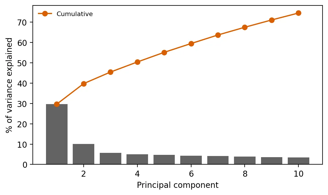Figure 1. The first principal component explains about 30% of the variation in burden, three times more than any other.

Component	What it captures (strongest loadings)
PC1: urban-industrial burden	Known contaminated sites (+0.33), air-permitted facilities (+0.32), surface heat (+0.32), impervious surface (+0.32), lack of tree canopy (+0.30), diesel PM (+0.28)
PC2: air toxics vs. legacy land contamination	Air toxics cancer (+0.47) and non-cancer (+0.38) risk vs. flooding (−0.36), deed notices (−0.33), contaminated-site areas (−0.32)
PC3: flooding vs. freight and ozone	Flooding (+0.31) vs. ozone, truck traffic, surface water, warehouses (about −0.3 each)

Almost every stressor loads positively on PC1. That makes it a natural data-driven burden index: higher PC1 means more of nearly everything at once. Notably, the heat measure from my earlier post is one of PC1’s strongest components, so heat belongs in conversations about cumulative burden.

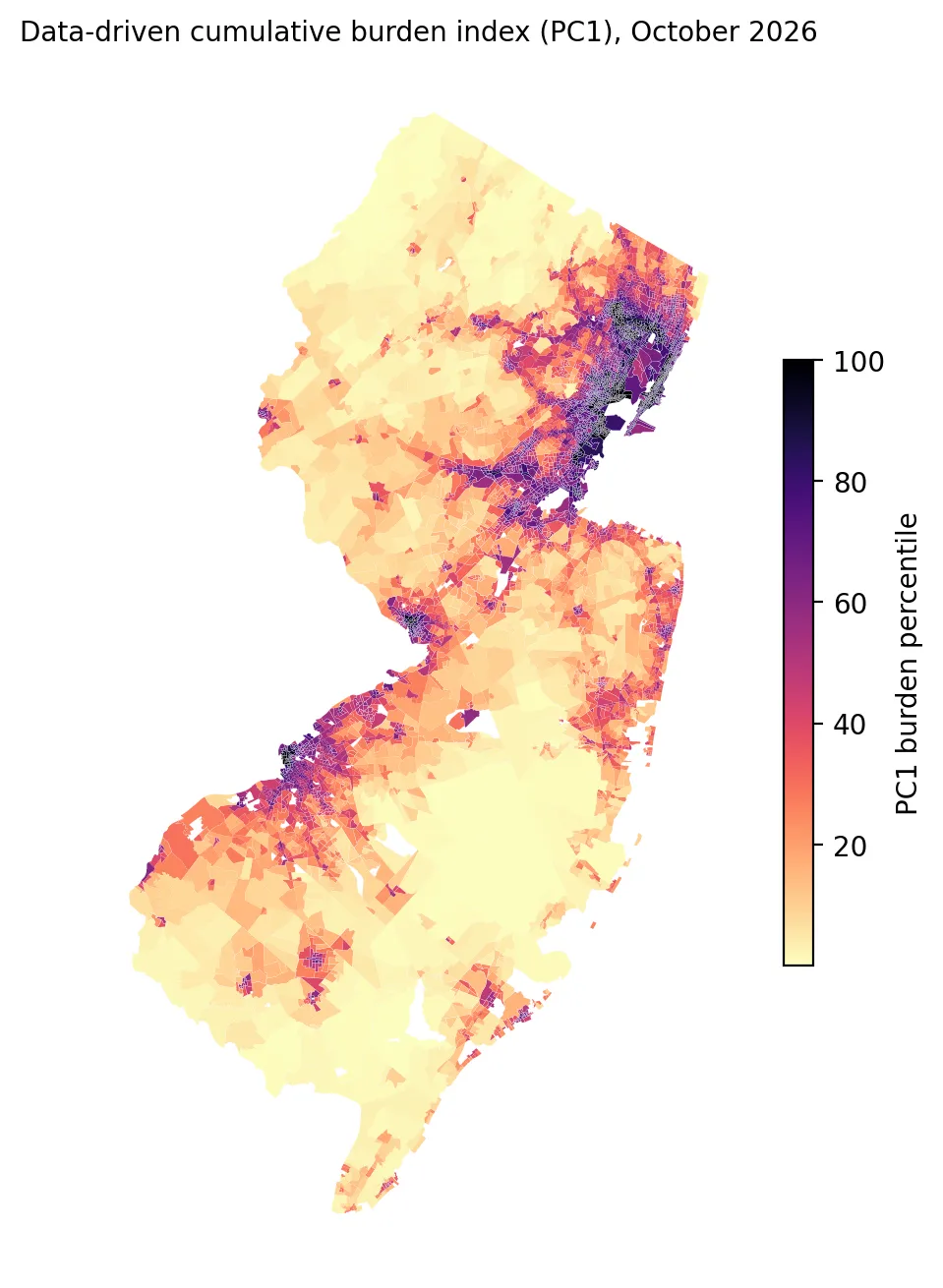Figure 2. A data-driven burden index is highest in northeastern New Jersey and other urban industrial areas.

Comparing with NJDEP’s count

PC1 and NJDEP’s Combined Stressor Total agree strongly (Spearman’s ρ = 0.80). Two very different methods, weighted versus counted, point to mostly the same places.

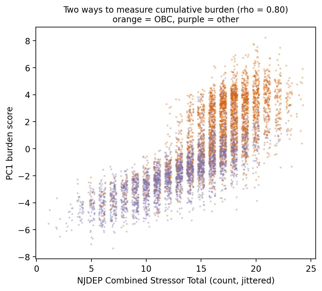Figure 3. The PC1 burden score and NJDEP’s stressor count largely agree on which places are most burdened.

• The top 20% of block groups by PC1 are home to 1.8 million people, and 95% of those block groups are overburdened communities.
• Only 68 non-OBC block groups (about 83,000 residents) are in the top 20%. These are highly burdened places that don’t meet the law’s income, minority, or language thresholds.
• At the other end, 702 OBCs are in the bottom 40% of PC1 burden. These communities qualify demographically but are comparatively less burdened environmentally, often suburban or rural low-income areas.
• Among OBCs, a simple “top half of PC1” rule agreed with NJDEP’s “adverse cumulative stressors” determination 84% of the time. NJDEP’s rule labels more OBCs as adverse (86% vs. 72%), partly because its comparison points are based on non-OBC medians.

Three kinds of burdened places

I used k-means clustering on the first four components to group block groups into types. The silhouette score, which measures how well-separated the groups are, was highest for three clusters (0.40):

Cluster	Block groups	Residents	OBC share	Average burden percentile	Distinctive traits
Legacy industrial	776	1.1 million	90%	81	Deed notices, contaminated sites, rail, scrap yards
Urban air and heat	2,126	2.8 million	83%	76	Diesel PM, air facilities, air toxics, impervious surface
Suburban / rural	3,489	5.3 million	33%	27	Flooding, surface water, truck traffic routes, regional PM2.5

This typology suggests that different burdened communities need different solutions: site cleanup and redevelopment controls in legacy industrial areas; diesel, traffic, and heat strategies in dense urban areas; and flood resilience in many lower-burden suburban and rural communities.

Looking back at earlier posts

This project began in October 2023 with a claim: environmental injustice exists in New Jersey (introduction). Forty posts later, the evidence for that claim comes from many directions:

1. Facilities are sited in overburdened communities. Residents of overburdened communities are far more likely to live next to trash incinerators (94% of residents within a mile), fuel-burning power plants (53% vs. 17% within three miles), toxic-release facilities (35% vs. 10% within a mile), chemical accident risks, scrap yards, and Superfund sites.
2. The gaps survive tougher tests. Comparing neighborhoods within the same county, overburdened communities still have about twice the contaminated-site density, 3.3 times the odds of a toxic-release facility nearby, and 2.1 times as many serious hazards. Poorer schools sit closer to highways even within counties.
3. Burdens pile up in the same places. One in three overburdened communities faces five or more serious hazards at once, compared with one in 25 other neighborhoods (my cumulative hazards post). This post’s burden index shows those hazards overlap: one main pattern (the first principal component) explains three times more of their variation than any other.
4. Race matters, not just income. For 11 of 12 environmental indicators, burdens are more concentrated by race than by income (my pollution inequality post), matching decades of national research.
5. The pattern reaches climate risks, too. Heat hot spots are 91% overburdened, and overburdened neighborhoods have far less tree canopy.

Along the way, checking what was known when mattered: map versions change, reports are delayed, crowd-sourced data are incomplete, and in February 2025 a major federal tool, EJScreen, was taken offline (my EJScreen post). Some results were smaller after stricter controls, and some measures still have gaps. Those details make the overall conclusion more convincing, not less: across air, land, water, heat, and the facilities themselves, New Jersey’s environmental burdens fall hardest on overburdened communities and communities of color.

Limitations

• PCA is descriptive. It finds patterns of co-occurrence, not causes or health risks, and PC1’s weights reflect how often stressors move together, not how harmful each one is.
• Variable choice shapes the result. Different inputs would produce a somewhat different index.
• Clusters are a simplification. A silhouette of 0.40 means the types are real but overlapping.

Code project (Level 6): PCA and clustering

Goal: Build a data-driven cumulative-burden index, compare it with NJDEP’s count-based approach, and identify community types.

Data: NJDEP EJ Law Combined Stressor Summary (Mar 31, 2026 version); outputs from my heat vulnerability and OpenStreetMap warehouse posts.

Method:

1. Assemble 26 measures; log-transform skewed ones; standardize.
2. Fit PCA; inspect explained variance (scree plot) and loadings.
3. Use PC1 as a burden index; compare with NJDEP’s CST and OBC status.
4. Run k-means on the first four components; choose k by silhouette score; profile each cluster.

from sklearn.decomposition import PCA
from sklearn.cluster import KMeans
Z = StandardScaler().fit_transform(X)
pca = PCA().fit(Z); pca.explained_variance_ratio_[:3]
labels = KMeans(3, n_init=10, random_state=34).fit_predict(Z @ pca.components_[:4].T)

New skills: dimension reduction, interpreting loadings, unsupervised clustering, and combining results from earlier projects into one analysis.

References

- New Jersey Department of Environmental Protection. (2026). Environmental Justice (EJ) Law Combined Stressor Summary (Current) [Data set]. https://www.arcgis.com/home/item.html?id=8f1eeb5074d147af8ab3e5e5a4f72d2b
- New Jersey Legislature. (2020). P.L.2020, c.92. https://pub.njleg.gov/bills/2020/PL20/92_.PDF
- OpenStreetMap contributors. (2026). OpenStreetMap [Data set, as of October 8, 2026]. https://www.openstreetmap.org/copyright
- Pedregosa, F., et al. (2011). Scikit-learn: Machine learning in Python. Journal of Machine Learning Research, 12, 2825–2830. https://jmlr.org/papers/v12/pedregosa11a.html
- U.S. Geological Survey. (2025). Landsat 8–9 Collection 2 Level-2 [Data set], via Microsoft Planetary Computer. https://planetarycomputer.microsoft.com/dataset/landsat-c2-l2